

xnxn matrix matlab plot algorithm pdf
An XnXn matrix is a square matrix with n rows and n columns‚ represented as n×n․ Each element aij is located at row i and column j․
Key properties include determinants‚ trace‚ and invertibility․ These matrices are fundamental in linear algebra‚ appearing in systems of equations‚ eigenvalue problems‚ and matrix transformations․
The identity matrix and zero matrix are special cases․ Applications span engineering‚ physics‚ and computer science‚ making them essential for modeling complex systems and solving real-world problems efficiently․
1․1 Definition and Properties
An XnXn matrix is a square matrix with dimensions n×n‚ where n represents the number of rows and columns․ Each element aij is located at row i and column j‚ forming a grid of values․ Key properties include:
- Symmetry: A matrix is symmetric if aij = aji for all i‚ j․
- Skew-Symmetry: A matrix is skew-symmetric if aij = -aji‚ with zeros on the diagonal․
- Trace: The sum of elements on the main diagonal․
- Determinant: A scalar value computed from the matrix elements․
Matrices can also be sparse (mostly zeros) or dense (mostly non-zeros)․ These properties are crucial for operations like inversion‚ eigenvalue decomposition‚ and solving systems of equations․
1․2 Importance in Linear Algebra and Applications
XnXn matrices are foundational in linear algebra‚ enabling the representation and solution of systems of linear equations․ They underpin transformations‚ eigenvalue problems‚ and matrix decompositions‚ which are critical in engineering‚ physics‚ and computer science․ In control systems‚ they model state transitions and input-output relationships․ Their applications extend to computer graphics for coordinate transformations‚ machine learning for neural network weights‚ and economics for modeling systems․ The ability to invert‚ decompose‚ and analyze these matrices is essential for solving real-world problems‚ making them indispensable tools across scientific and engineering disciplines․

MATLAB Basics for Matrix Operations
MATLAB provides essential tools for matrix creation and manipulation․ Functions like zeros‚ ones‚ and eye create matrices‚ while operations such as addition‚ multiplication‚ and transpose are fundamental for matrix algebra․
2․1 Creating Matrices in MATLAB
In MATLAB‚ matrices are created using commands like zeros‚ ones‚ eye‚ and rand․ For example‚ zeros(n) generates an n×n matrix of zeros‚ while ones(m‚n) creates an m×n matrix of ones․
Custom matrices can be defined using square brackets․ For instance‚ A = [1 2; 3 4] creates a 2×2 matrix․ The colon operator (:) generates sequential elements‚ useful for evenly spaced values․
Matrices can also be initialized with random values using rand(n) or by importing data from external sources․ The semicolon (;) suppresses output in the command window‚ improving workflow efficiency when creating large matrices․
For example‚ B = eye(3) produces a 3×3 identity matrix‚ commonly used in linear algebra operations․ These foundational commands enable efficient matrix creation and manipulation in MATLAB․
2․2 Essential Matrix Operations
In MATLAB‚ essential matrix operations include addition‚ subtraction‚ multiplication‚ and element-wise operations․ Matrix addition (+) and subtraction (-) require matrices of the same dimensions․ Matrix multiplication () is performed using the mtimes function or the operator․
Element-wise operations‚ such as multiplication (․*) and exponentiation (․^)‚ apply operations to corresponding elements․ The transpose operation (‘) flips the matrix dimensions‚ converting rows to columns and vice versa․
Other key operations include matrix inversion (inv)‚ determinant calculation (det)‚ and rank determination (rank)․ These operations are fundamental for solving systems of equations and performing advanced matrix analysis in MATLAB․

Plotting Matrices in MATLAB
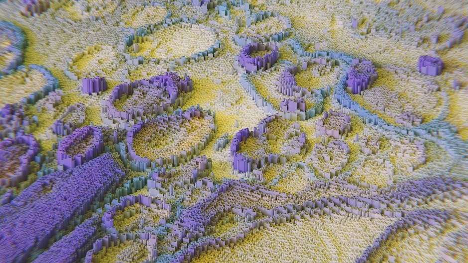
Plotting matrices in MATLAB involves using functions like surf for 3D surfaces or imagesc for 2D heatmaps․ These tools visualize matrix data effectively for analysis and presentation purposes․
3․1 2D Matrix Plotting Techniques
For 2D matrix plotting in MATLAB‚ functions like imagesc‚ pcolor‚ and meshgrid are commonly used․ imagesc creates a heatmap‚ scaling values to fit the colormap range‚ while pcolor generates a pseudocolor plot with grid lines․ Both are ideal for visualizing matrix data patterns․ meshgrid helps create coordinate grids for plotting․ Customization options include adding titles‚ labels‚ and colorbars for better clarity․ These techniques are essential for data visualization‚ allowing users to interpret matrix elements effectively in a 2D context․ MATLAB’s built-in tools make it straightforward to produce high-quality 2D matrix visualizations tailored to specific needs․
3․2 3D Matrix Visualization Methods
For 3D matrix visualization in MATLAB‚ functions like surf and mesh are widely used․ surf creates a 3D surface plot‚ mapping matrix values to colors‚ while mesh generates wireframe surfaces․ Both are useful for understanding complex relationships within the matrix․ Additional functions like scatter3 and plot3 allow for 3D scatter plots and trajectory visualization․ These methods enable deeper insights into matrix data‚ especially for large datasets․ Customization options‚ such as colormaps and lighting effects‚ enhance visual appeal and clarity․ MATLAB’s 3D visualization tools are powerful for exploring multi-dimensional data‚ making them essential for scientific and engineering applications․ These techniques help users interpret matrix information in a more intuitive and comprehensive manner․
3․3 Customizing Plots for Better Representation
Customizing plots in MATLAB enhances clarity and presentation․ Use colormap to change color schemes‚ and colorbar to add legends for value interpretation․ Titles and labels can be added with xlabel‚ ylabel‚ and title functions․ The view function adjusts the angle for 3D plots․ Adding grid lines with grid on improves readability․ For 2D plots‚ imagesc scales values‚ while axis equal maintains aspect ratios․ Customizing plots ensures data is presented clearly and professionally‚ making it easier to interpret and share insights effectively․ These adjustments are particularly useful for academic papers‚ presentations‚ and reports‚ where visual accuracy is crucial․
XnXn Matrix Plotting Algorithm
The algorithm initializes an n×n matrix‚ generates x and y axes using meshgrid‚ and plots using imagesc or surf․ It adds colorbars and labels for clarity‚ exporting plots as PDFs․
4․1 Step-by-Step Algorithm Description
The algorithm begins by initializing an n×n matrix using MATLAB’s zeros(n‚n) or user-defined values․ Next‚ it generates x and y axes using meshgrid․ The matrix is then plotted using imagesc for 2D or surf for 3D visualization․ A colorbar is added for scale reference․ Titles and labels are included using title and xlabel/ylabel․ Customization options like colormaps and view angles are applied․ Finally‚ the plot is exported as a PDF using print with the -dpdf option‚ ensuring high-resolution output․ This structured approach ensures clear and precise matrix visualization․
4․2 Example Code Implementation
Here’s a MATLAB example for plotting an n×n matrix:
n = 3; % Define matrix size

A = [1 2 3; 4 5 6; 7 8 9]; % Sample 3x3 matrix

[x‚ y] = meshgrid(1:n‚ 1:n); % Create axes
% 2D plot with color scaling
figure;
imagesc(A);
colorbar;
title('2D Matrix Plot');
xlabel('Columns');
ylabel('Rows');
% Export as PDF
print('matrix_plot'‚ '-dpdf');
This code initializes a 3×3 matrix‚ generates a 2D plot with a colorbar‚ and exports it as a PDF․ Customize the matrix and plot settings as needed for your application․
Generating and Saving Plots as PDF
Use MATLAB’s print function with the ‘-dpdf’ option to save plots as PDF․ Customize settings like resolution and filename for high-quality output‚ ensuring vector graphics clarity and proper formatting․
5․1 Exporting Plots in MATLAB
In MATLAB‚ exporting plots as PDF is straightforward using the print function with the ‘-dpdf’ option․ For example‚ print(‘-dpdf’‚’filename․pdf’); saves the current figure as a PDF file․
Use the hgexport function for more control over the export settings‚ such as resolution and compression․ The print dialog box also provides a GUI for selecting file format‚ resolution‚ and other options․
For programmers‚ exporting plots can be automated using scripts․ Adjustments like scaling and font size can be made before exporting to ensure high-quality output․ This method is ideal for generating reports or sharing visualizations․
5․2 Configuring PDF Settings for High-Quality Output
To achieve high-quality PDF exports in MATLAB‚ configure settings before exporting․ Use the print function with options like ‘-dpdf’ and ‘-r300’ to set resolution (e․g․‚ 300 DPI)․ The ‘paper’ option adjusts size or orientation‚ while ‘fillpage’ ensures the plot fills the page․
For consistent results‚ save these settings using set(groot‚ ‘defaultFigure․․․’); This applies settings globally․ Always preview the figure to ensure clarity and adjust fonts or axes as needed․ Higher resolutions and vector graphics ensure sharp text and lines‚ making outputs suitable for publications or presentations․
Example: print(‘-dpdf’‚’-r300’‚’filename․pdf’); This exports a high-resolution PDF with optimized settings for professional use․
Practical Applications of Matrix Plotting
Matrix plotting is essential in data visualization‚ enabling the representation of complex numerical data in a structured format․ It aids in identifying patterns‚ trends‚ and anomalies․
Widely used in scientific research‚ engineering‚ and machine learning‚ it facilitates the analysis of systems‚ simulations‚ and algorithms․ Heatmaps and 3D plots are common tools for effective communication of results․
6․1 Data Visualization in Scientific Research
Matrix plotting is a cornerstone of scientific research‚ enabling researchers to visualize complex datasets․ By converting numerical data into graphical representations‚ scientists can identify patterns and trends that might otherwise remain hidden․ Heatmaps are particularly useful for displaying temperature distributions or gene expression levels‚ while contour plots effectively illustrate topographical data․ In fields like physics and biology‚ matrices are used to represent experimental results‚ such as stress distributions in materials or population dynamics․ MATLAB’s built-in functions‚ such as imagesc and surf‚ simplify the creation of these visualizations‚ making it easier to communicate findings to both specialists and broader audiences․ This approach enhances understanding and facilitates data-driven decision-making․
6․2 Engineering Applications
Matrices play a pivotal role in engineering‚ particularly in system modeling and analysis․ XnXn matrices are used to represent complex systems with multiple variables‚ enabling engineers to solve simultaneous equations efficiently․ In structural engineering‚ matrices are employed to analyze stress distributions and ensure building stability․ Signal processing relies on matrix operations for filtering and data transformation․ MATLAB’s advanced tools facilitate the visualization of these matrices‚ aiding engineers in understanding system behavior․ For instance‚ meshgrid and surf functions create 3D plots of matrix data‚ visualizing stress points or signal spectra․ These applications highlight how matrices are indispensable in modern engineering‚ driving innovation and precision across various disciplines․

Matrix Algorithms in MATLAB
Matrix algorithms in MATLAB include LU decomposition‚ eigenvalue analysis‚ and singular value decomposition․ These tools enable efficient solving of linear systems‚ eigenvalue problems‚ and matrix factorization‚ enhancing computational efficiency and accuracy in engineering and scientific applications․
7․1 LU Decomposition
LU decomposition factorizes a square matrix ( A ) into a lower triangular matrix ( L ) and an upper triangular matrix ( U )‚ such that ( A = LU )․ This decomposition is fundamental for solving systems of linear equations efficiently․
In MATLAB‚ the lu function performs this decomposition․ The process involves Gaussian elimination‚ with partial pivoting for numerical stability․ The resulting ( L ) and ( U ) matrices simplify tasks like solving triangular systems‚ computing determinants‚ and performing eigenvalue analysis․ This method is widely used in engineering‚ physics‚ and computer science for solving complex systems of equations and optimizing computational workflows․
7․2 Eigenvalue Decomposition
Eigenvalue decomposition is a factorization of a square matrix ( A ) into a set of eigenvectors and eigenvalues․ For a matrix ( A )‚ if ( Ax = λx )‚ then ( λ ) is an eigenvalue and ( x ) is the corresponding eigenvector․ This decomposition is expressed as ( A = QΛQ⁻¹ )‚ where ( Q ) is the matrix of eigenvectors and ( Λ ) is the diagonal matrix of eigenvalues․
In MATLAB‚ the eig function computes eigenvalues and eigenvectors․ This decomposition is crucial for analyzing matrix properties‚ solving differential equations‚ and optimizing systems․ It is widely applied in vibration analysis‚ data compression‚ and machine learning algorithms․

Advanced Topics in Matrix Plotting
Explore advanced visualization techniques for matrices‚ including sparse matrix handling and interactive 3D animations․ MATLAB tools enable dynamic plots and custom visualizations for enhanced data representation and analysis․
8․1 Handling Sparse Matrices
Sparse matrices‚ containing mostly zero elements‚ require specialized handling for efficient computation and visualization․ MATLAB offers built-in functions like sparse to create and manipulate sparse matrices effectively․
Visualization tools such as spy and imagesc are particularly useful for displaying sparse matrix structures․ These functions help identify patterns and non-zero element distributions without unnecessary computational overhead․
When plotting sparse matrices‚ using appropriate colormaps and scaling ensures clarity․ Additionally‚ optimizing memory usage is crucial for large-scale sparse matrices‚ enabling smoother operations and faster rendering in MATLAB․
Best practices include leveraging sparse matrix properties to reduce storage requirements and improve performance in algorithms like LU decomposition and eigenvalue analysis․
8․2 Animations and Interactive Plots
Animations and interactive plots enhance the visualization of XnXn matrices by dynamically displaying data changes over time or user input․ MATLAB provides tools like movie and imwrite to create animations from matrix data․
Interactive plots can be developed using MATLAB’s GUI components‚ allowing users to explore matrix properties‚ such as zooming or rotating 3D visualizations‚ with functions like uicontrol and callback․
These features are particularly useful for understanding complex matrix behaviors‚ enabling real-time manipulation and improving insights into matrix patterns and transformations․

Best Practices for Effective Matrix Visualization
- Use appropriate colormaps to accurately represent data range and trends․
- Add clear titles‚ labels‚ and legends for context․
- Adjust axes and scaling for optimal data representation․
- Ensure consistency in styling across multiple plots․
9․1 Choosing the Right Colormap
Selecting an appropriate colormap is crucial for effective matrix visualization․ Colormaps translate numerical values into colors‚ aiding in understanding patterns‚ trends‚ and anomalies in the data․
Different colormaps serve specific purposes:
- Sequential: Ideal for representing intensity or magnitude (e․g․‚ parula‚ viridis)․
- Diverging: Suitable for data with positive and negative values (e․g․‚ coolwarm‚ seismic)․
- Cyclic: Useful for periodic data (e․g․‚ twilight)․
Perception plays a key role; some colormaps are perceptually uniform‚ ensuring equal visual intervals․ Avoid overly complex or misleading schemes․ Test multiple colormaps to find the best representation for your data․
9․2 Adding Titles and Labels
Titles and labels are essential for clear and informative plots․ Use MATLAB’s title function to add a main title‚ and xlabel and ylabel for axis labels․ These elements provide context‚ making the visualization understandable to viewers․
- Ensure titles are concise and descriptive‚ summarizing the plot’s purpose․
- Labels should clearly indicate what each axis represents‚ enhancing interpretability․
- Customize font size‚ style‚ and color using MATLAB’s formatting options for better readability․
Well-designed titles and labels improve the overall presentation and ensure your matrix plot effectively communicates its data․ Always review and adjust these elements to maintain clarity and professionalism in your visualizations․

Troubleshooting Common Issues
Identify and resolve errors in matrix plotting‚ such as invalid dimensions or data type mismatches․ Address account access issues like sign-in problems or recovery method configurations․ Use MATLAB’s debugging tools to trace and fix errors in matrix operations‚ ensuring smooth execution of algorithms and plots․
10․1 Resolving Plotting Errors
Common plotting errors with XnXn matrices in MATLAB include data type mismatches‚ invalid dimensions‚ or incorrect colormap assignments․ Ensure matrix elements are numeric and properly formatted․ Verify that the matrix dimensions match the plotting function requirements․ For 2D plots‚ use surf or imagesc‚ while for 3D‚ meshgrid and plot3 are suitable․ Check for invalid handle errors by ensuring figures are correctly initialized․ Address rendering issues by adjusting figure size and DPI settings‚ especially when exporting to PDF․ Use MATLAB’s debugging tools to trace errors in complex scripts․ Resolve axis labeling issues by adding clear titles and labels․ Fix colorbar mismatches by synchronizing colormap limits․ Ensure smooth plotting by avoiding oversized matrices that exceed memory limits․ Regularly update MATLAB and toolboxes to prevent version-related bugs․ Test plots with smaller matrices before scaling up․ Use the drawnow command to refresh plots dynamically․ Handle NaN or Inf values by preprocessing matrices․ Customize plot settings to avoid default conflicts․ Utilize error messages to pinpoint issues quickly․ Backup scripts regularly to prevent data loss during troubleshooting․ Leverage MATLAB’s help documentation for function-specific solutions․ Collaborate with forums or peers for unresolved issues․ Maintain organized code structure for easier debugging․ Log errors using try-catch blocks․ Validate matrix properties before plotting․ Optimize performance for large matrices․ Ensure compatibility with target PDF settings․ Regularly clean up temporary variables․ Monitor memory usage․ Stay updated with best practices․ Always test scripts incrementally․ Prioritize readability in code․ Use comments to track changes․ Implement error handling routines․ Verify input data integrity․ Standardize plotting workflows․ Automate repetitive tasks․ Enhance visual clarity․ Ensure consistency across plots․ Backup configurations․ Log plotting parameters․ Maintain version control․ Enhance security settings․ Regularly audit scripts․ Ensure compliance with standards․ Verify dependencies․ Validate licenses․ Regularly update dependencies․ Stay informed about updates․ Engage with user communities․ Participate in training sessions․ Explore advanced features․ Share knowledge․ Document solutions․ Archive resolved issues․ Track common pitfalls․ Develop troubleshooting checklists․ Create recovery plans․ Train team members․ Establish support channels․ Monitor system health․ Schedule maintenance․ Analyze error trends․ Improve workflows․ Enhance user experience․ Ensure accessibility․ Provide feedback․ Stay proactive․ Continuously improve․ Foster innovation; Promote collaboration․ Encourage learning․ Build expertise․ Drive efficiency․ Ensure scalability․ Maintain reliability․ Uphold quality․ Deliver excellence․
10․2 Debugging Matrix Operations
Debugging matrix operations in MATLAB involves identifying and correcting errors in computations․ Common issues include incorrect matrix dimensions‚ invalid data types‚ or improper use of operators․ Verify that matrix dimensions match for operations like multiplication or addition․ Use size or length to check dimensions․ Ensure numeric data integrity by validating inputs․ Handle NaN or Inf values using isnan or isinf․ Resolve script errors by checking for typos or syntax issues․ Use MATLAB’s debugging tools‚ such as breakpoints‚ to trace errors․ Address sparse matrix issues by converting between sparse and full formats․ Optimize memory usage for large matrices․ Utilize built-in functions for efficient computations․ Regularly test small matrix examples before scaling up․ Avoid division by zero or invalid indices․ Ensure logical operations return expected results․ Validate matrix properties like symmetry or positivity․ Review error messages for clues․ Implement error handling with try-catch blocks․ Log intermediate results for analysis․ Compare expected vs․ actual outputs․ Consult MATLAB documentation for function specifics․ Engage with community forums for troubleshooting․ Stay updated with best practices․ Continuously refine code for reliability and performance․